Visualize Project Data

If the user needs to visualize the recorded and processed project data in 1D, 2D or 3D the Visualize Project Data functions will need to be used.

Select the "Visualize Project Data" option from the Project Data menu. The full menu can be seen by left swiping the Project data options bar. Right swiping will close the full option menu.

To view the 1D of any project point with processed data available, select the 1D tab. Under the View Tab, select a point to view in the Select point list.

Then select a data set to view for that point. There are 27 possible data sets available.

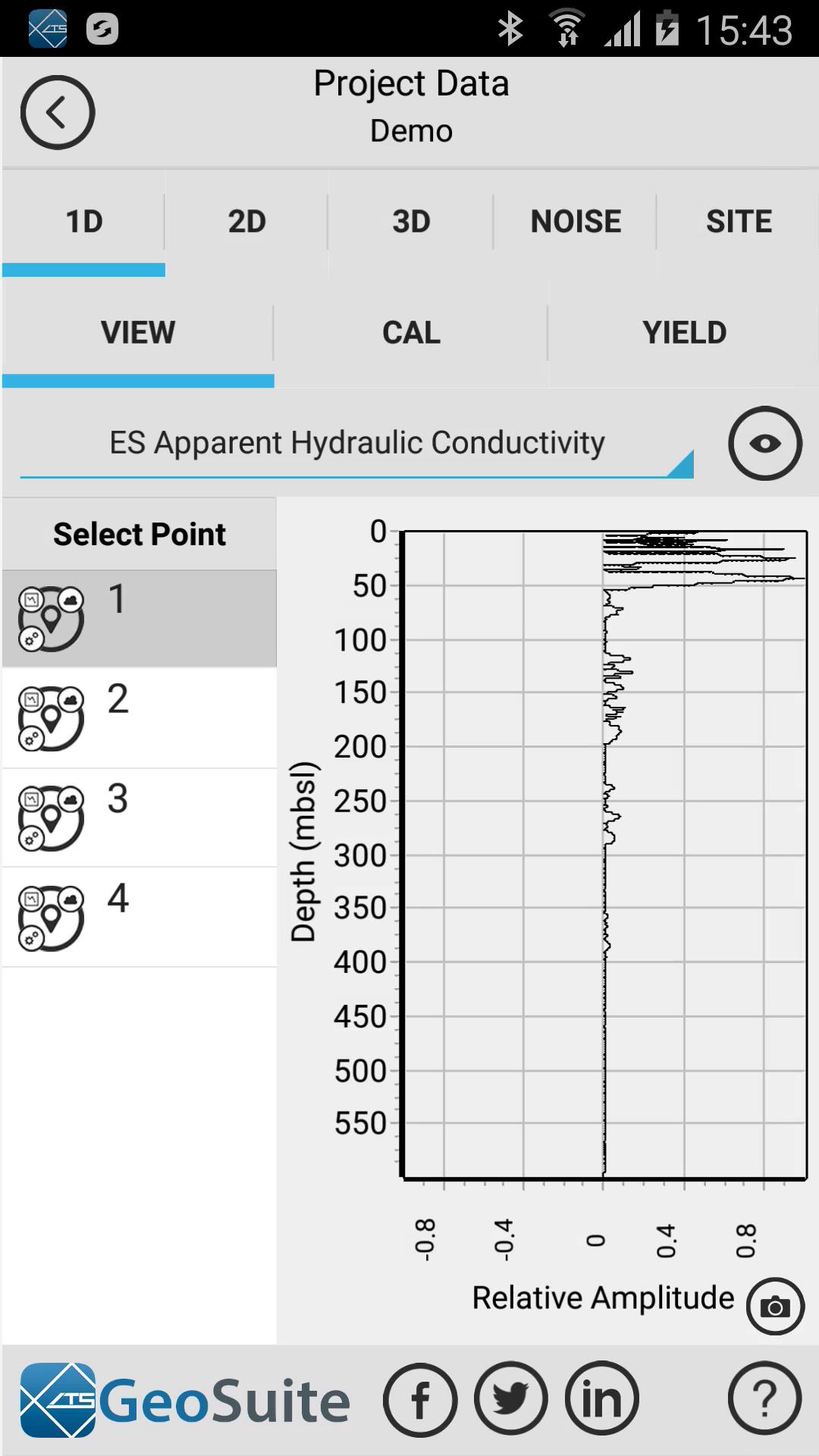
To take a snapshot of the 1D chart select the snapshot option on the chart. One selected, a PDF document containing an image of the current chart will be saved to the Documents folder on the device. A snapshot option exists on the 2D and 3D chart as well

To view 2D data for a set of project points, select the 2D tab. Under the setup tab, select the project points, in order of position, in the Select Data point list. Select a data set which you want to view for the points, 27 possible data sets are available. The user may use the default interpolation, contouring, depth, elevation correction and color scheme settings or modify them to personalized settings. If calibration data is available, this may also be applied by selecting the calibration point to apply Once done, select the render button.

The Grid and interpolation properties provided to the user are:

Lateral Grid : the number of lateral grid points to be rendered

Vertical Grid : the number of vertical grid points to be rendered

Lateral Radius : the 2D lateral interpolation search radius distance, in meters

Vertical Radius : the 2D vertical interpolation search radius distance, in meters

Contours : the number of individual contours to include in the 2D rendering

Max Depth : the depth to which the 2D data is to be rendered to

SRTM corrected elev : use SRTM elevation data in the 2D rendering instead of the default GPS sensor elevation data.

Auto search radius : This option, active by default, will atomatically determin the best lateral interpolation radius to apply to the data set when the 2D image is rendered.

Clip Data : the maximum amplitude, expressed as a percentage of the maximum data amplitude for all of the included points in the 2D rendering, to which the 2D data set is to be rendered.

2D Gridding

Almost all ES data is originally in the form of an irregular grid format, in which the survey points do not conform to a perfect grid with exactly equal distance between survey points. The survey points also almost always have variations in elevation between survey points. In order to interpolate the data to create the 2D contours needed to visualize the ES data, this irregular grid data must first be turned in to a regular grid.

This regular grid format is by default set to a grid layout of 25 by 100 grid points in the Lateral,  Vertical directions. All data generated is referenced to this regular grid.

The:

1) Lateral Grid

2) Vertical Grid

Allow the user to changes these grid setting in order to increase or decrease the rendered resolution of the contour data. The benefit of increasing the Grid settings is improved model resolution in the lateral and vertical scales. This will allow the user to see more detail in the model as there are more individual grid points to visualize. Increasing the resolution of the model will significantly affect the rendering performance of the interactive 2D contour chart within the app. This is due to the fact that there are more data points to render.

The absolute resolution of the 2D contour plot, as defined by the grid step settings in the Lateral,  and Vertical direction and the current 2D plot boundaries. For example, if the render depth (set by the Max Depth field) is set to be 100 meters and the Vertical Grid field is set to be 100, then the absolute resolution of the gridded model will be 1 meter.

This is calculated using the following equation.

Absolute Vertical Resolution = Max Depth / Vertical Grid

The same calculation is true for the Lateral grid setting.

2D Interpolation

The interpolation strategy used to create3D objects shown in the 2D contour plot is the Inverse distance method. The interpolation strategy uses an Isotropic Anisotropy by default with a drop-off power of 2. The lateral interpolation distance is calculated as the longest distance between any two adjacent points within the project data set. This value defines the search radius with which to include data points to apply to the interpolation process.

This distance is calculated automatically on loading the 2D tools tab.

This ensures that all the points in the model interpolate with at least one other neighboring point. The vertical interpolation distance is by default set to 5m for all the data sets in the model.

This effectively gives all the model data sets an effective vertical resolution of 5m.

The user may edit the lateral and vertical interpolation search radius by editing the values in the following fields:

1) Lateral Radius

2) Vertical Radius

Increasing these values will affect the gridding and rendering speed of the 2D contour plot within the app.

Clip Data

To increase the sensitivity of the, rendered 2D, data set amplitude, use the Clip Data slider. This value expresses the maximum amplitude value, as a percentage of the maximum data value for all the points included in the 2D rendering, that the 2D rendering is to be rendered to. So effectively, by dropping the clipping value to 50% the 2D rendering amplitude sensitivity will be doubled.

This is done to visually enhance rendered 2D data features on the contour plot, that were not immediately visible using a 100% clip Data value.

Max Depth

The max depth field provided in the app defines the maximum depth below surface level to which the 3D data plots is to be rendered.

Once the data has rendered, select the View tab to see the resultant 2D data set.

To visualize project point data in 3D, select the 3D tab.

The 3D render engine requires gridding of the data to be performed before any data can be visualized in 3D. To do this, select the gridding tab. Select the point which are to be included in the gridding data set, under the Project Points list. If a calibration data set is to be added, select the calibration point to apply to the gridding data under the Calibration Points list. The user may use the default interpolation, elevation correction and gridding depth settings to generate the gridding data set. Or the user may choose to customize these settings. Lastly select the data sets which you would like to generate gridding data for. There are 27 data sets available for gridding.

The 3D gridding options include:

1) Latitude Grid Steps - The number of gridding points in the latitudinal direction.

2) Longitude Grid Steps - The number of gridding points in the longitudinal direction

3) Depth Grid Steps - The number of Gridding points in the vertical direction.

4) Data Set Increment - The number of real data points to skip when generating the 3D grid.

5) Lateral Radius - The lateral search radius used in the interpolation scheme.

6) Vertical Radius - The vertical search radius used in the interpolation scheme.

7) Max Depth - The maximum depth below surface level to which the 3D data plots is to be rendered.

3D Gridding

Almost all ES data is originally in the form of an irregular grid format, in which the survey points do not conform to a perfect grid with exactly equal distance between survey points. The survey points also almost always have variations in elevation between survey points. In order to interpolate the data to create the 3D objects needed to visualize the ES data, this irregular grid data must first be turned in to a regular grid.

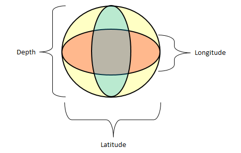
This regular grid format is by default set to a grid layout of 10 by 10 by 10 grid points in the Latitude, Longitude and Depth directions. All data generated is referenced to this regular grid.

The:

1) Latitude Grid Steps

2) Longitude Grid Steps

3) Depth Grid Steps

Allow the user to changes these grid setting in order to increase or decrease the rendered resolution of the model data. The benefit of increasing the Grid step settings is improved model resolution in the lateral and vertical scales. This will allow the user to see more detail in the model as there are more individual grid points to visualize. Increasing the resolution of the model will significantly affect the rendering performance of the interactive 3D model chart within the app. This is due to the fact that there are far more data points to render.

The absolute resolution of the 3D model as defined by the grid step settings in the Latitude, Longitude and Depth direction and the current model boundaries. For example, if the render depth (set by the Max Depth field) is set to be 100 meters and the Depth Grid Steps field is set to be 10, then the absolute resolution of the gridded model will be 10 meters.

This is calculated using the following equation.

Absolute Depth Resolution = Max Depth / Depth Grid Steps

The same calculation is true for the Longitude and Latitude grid step settings.

3D Interpolation

The interpolation strategy used to create3D objects shown in the 3D modelis the Inverse distance method. The interpolation strategy uses an Isotropic Anisotropy by default with a drop-off power of 2. The lateral interpolation distance is calculated as the longest distance between any two adjacent points within the project data set. This value defines the search radius with which to include data points to apply to the interpolation process.

This distance is calculated automatically on loading the 3D tools tab.

This ensures that all the points in the model interpolate with at least one other neighboring point. The vertical interpolation distance is by default set to 5m for all the data sets in the model.

This effectively gives all the model data sets an effective vertical resolution of 5m. This effectively warps the shape of the interpolation shape to that of a flattened sphere.

The user may edit the lateral and vertical interpolation search radius by editing the values in the following fields:

1) Lateral Radius

2) Vertical Radius

Increasing these values will affect the gridding and rendering speed of the 3D model within the app.

Data Set Increment

The data set increment setting in the app is defined as the number of real data points to skip when generating the 3D grid. So in essence, setting this value to 10 will effectively only include every tenth real data point into the interpolation process during the gridding of the model data.

This is done to improve the interpolation performance of the gridding process as less data is required to grid the model.

The downside of increasing this value is that the resolution of the real point data is decreased.

Max Depth

The max depth field provided in the app defines the maximum depth below surface level to which the 3D data plots is to be rendered.

Once all the options and settings have been completed, select the Generate Gridding Data button to generate the gridding data files.

Once the Gridding data has been created, the data sets generated can be visualized in 3D. to do this select the Render tab. Under the Select Data Sets to Render list, select the data sets you would like to include in the 3D model. To modify the default data set variables select the data set you wish to modify in the Select Data Sets to Render list, the current values will show in the Render Model data section. The user may use the default values or change the ISO-surface value, color, transparency and border view settings. To save the changes to the data set settings press the refresh button.

To render the 3D model, click on the Render Model Data button.

Once the 3D model data has rendered, select the Model tab to view the rendered 3D Model. The model is interactive and can be rotated and zoomed.

To Visualize the noise and quality control statistics data collected for a project in 2D, select the "Noise" Tab.

Now select the Noise or Quality control data set you want to render.

Now render and view the data.

To visualize site specific 2D data such as site elevation, magnetic data or soil resistivity data, select the "Site" tab.

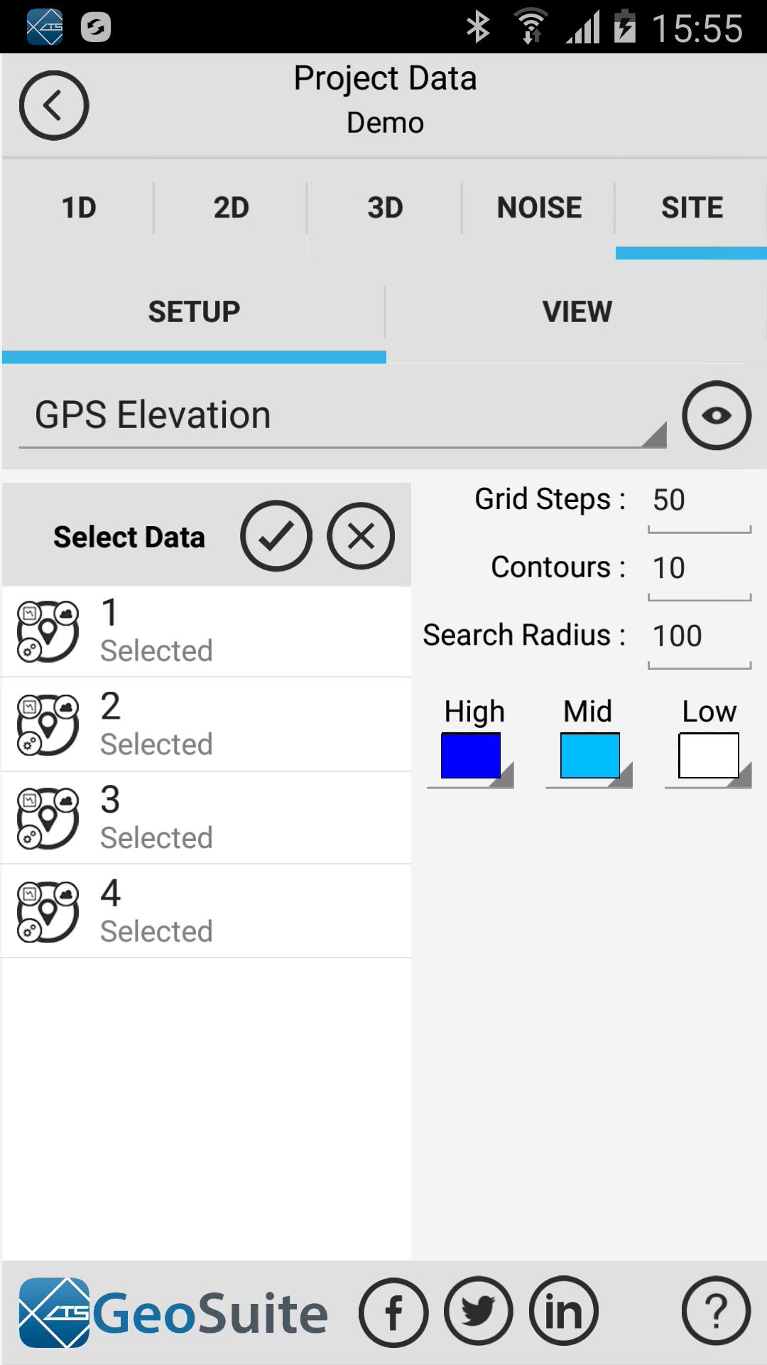
Select the data set you wish to render.

Then select the render option and view.